Bayesian Optimization · Active Learning · Materials Discovery

2026 — ongoing

After building the inverse design engine, I kept running into the same frustration. The generation step and the validation step were disconnected. You specify target properties, the engine generates candidates, the NNP screens them, Reformix validates the best ones, and then you stop. The results from the validation runs, the actual simulated properties of the candidates you evaluated, went nowhere. They did not feed back into anything. Every simulation you run tells you something about the property landscape, about which molecular features correlate with which thermomechanical behaviors, and that information was just being discarded.

That felt wrong. If you are going to spend compute on simulating a candidate, the result should make your next candidate better, not just confirm or deny the current one.

This is what active learning loops are designed to do. The idea has been around in statistics for decades under different names: sequential experimental design, Bayesian optimization, optimal experiment design. The core principle is the same. You have a space of possible inputs, a function mapping inputs to outputs that is expensive to evaluate, and a budget of evaluations. You want to find the best input using as few evaluations as possible. Instead of evaluating inputs at random or exhaustively, you build a model of the function from the data you have, use that model to predict where the best inputs are likely to be, and evaluate there next. Then you update the model with the new result and repeat.

In the Reformix context, the expensive function is molecular simulation. The input is a candidate formulation, defined by its resin type, hardener type, molecular weight, and stoichiometry. The output is a set of thermomechanical properties. The budget is compute time. The goal is to find formulations with target properties using as few full simulation runs as possible.

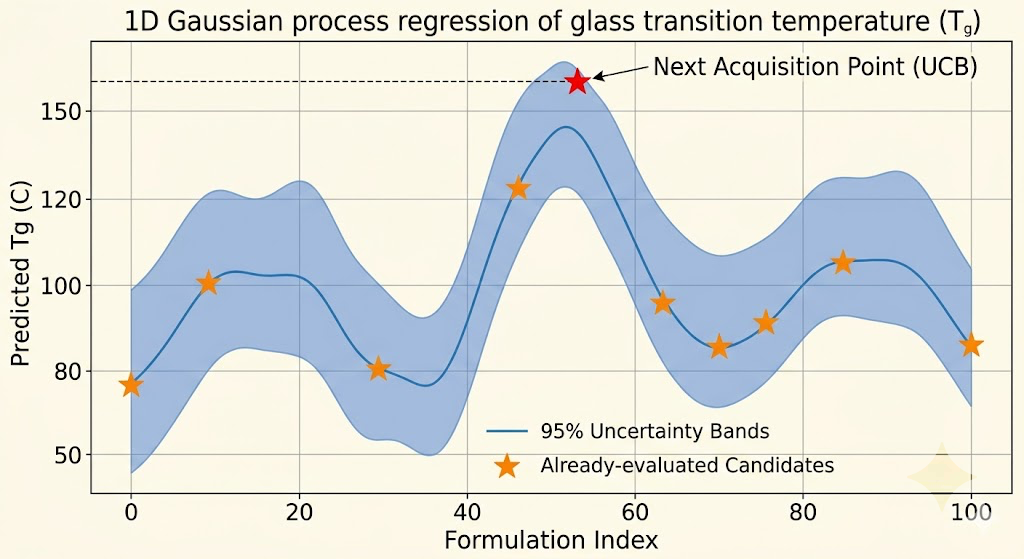
The surrogate model I use is a Gaussian process. Gaussian processes are well-suited for this application for a specific reason: they produce calibrated uncertainty estimates alongside their predictions. For every candidate formulation you ask about, the GP tells you both its best guess at the properties and how confident it is in that guess. That uncertainty is what makes intelligent exploration possible.

The acquisition function is the part that actually decides what to simulate next. It takes the GP's predictions and uncertainties over all candidate formulations and scores each one according to a policy that balances two competing objectives. Exploitation means evaluating candidates where the GP predicts good properties, because those are likely to actually be good. Exploration means evaluating candidates where the GP is uncertain, because those might be even better and the uncertainty will decrease regardless of the result. A policy that only exploits converges to a local optimum. A policy that only explores wastes compute on uninformative regions. The standard approach, upper confidence bound acquisition, scores each candidate as its predicted mean plus a constant times its predicted standard deviation, and that constant controls the exploration-exploitation tradeoff.

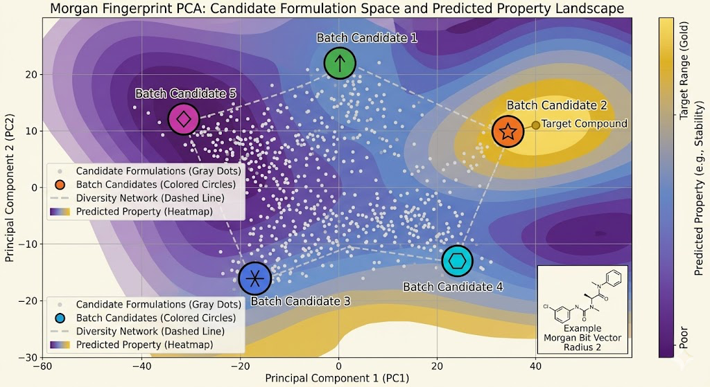
The input representation for the GP matters a lot. Raw molecular structures are high-dimensional and the GP kernel needs to measure similarity between them meaningfully. I use molecular fingerprints as the input representation, specifically Morgan fingerprints at radius 2, which capture the local chemical environment around each atom out to two bonds away. Two molecules with similar fingerprints have similar local chemistry, and similar local chemistry tends to produce similar macroscopic properties. The GP kernel over fingerprint space is a Tanimoto kernel, which is the standard similarity measure for molecular fingerprints and behaves better than Euclidean distance for this kind of bit vector representation.

The loop itself runs as follows. Start with an initial dataset of simulated formulations, in my case the Reformix validation results and the NNP-screened candidates from the inverse design pipeline. Train the GP on this dataset. Use upper confidence bound acquisition to score all candidate formulations in a defined search space. Select the top-scoring candidate. Run it through the NNP for fast property estimation. If the NNP result looks promising, escalate to full Reformix simulation. Add the result to the dataset. Retrain the GP. Repeat.

The escalation step between NNP and full simulation was something I added after the first few iterations of the loop because running full Reformix on every acquisition-selected candidate was still too expensive. The NNP acts as a cheap filter. If the NNP predicts properties outside the target range, the candidate gets rejected without spending compute on full simulation. Only candidates that pass the NNP screen get escalated. This creates a two-stage evaluation pipeline: fast screening with the NNP, expensive validation with Reformix. The active learning loop drives the selection at the top, and the two-stage evaluation handles the budget.

Batch acquisition was necessary once I realized that running one candidate at a time and retraining the GP after each result was too slow. The GP retraining is fast relative to simulation, but you still want to be running multiple simulations in parallel to use the available compute efficiently. Batch Bayesian optimization selects a set of candidates simultaneously rather than one at a time, with the constraint that the batch should be diverse: candidates that are similar to each other in the fingerprint space provide redundant information, so the batch should cover different regions of the search space. I use a greedy approach where you select the first candidate by acquisition score, then reduce the scores of nearby candidates using the expected information gain from the first selection, then select the second candidate from the adjusted scores, and so on until the batch is full.

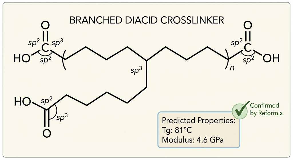
The first result that genuinely surprised me came in the third loop iteration. The GP selected a candidate with a non-standard crosslinker architecture that I would not have thought to propose manually, a branched diacid with a longer chain than the simple systems in the initial dataset. The NNP predicted a Tg of 83°C and a modulus of 4.8 GPa, both above the target values. Full Reformix simulation confirmed: Tg of 81°C, modulus of 4.6 GPa. That candidate went into the patent pipeline.

The loop has now run through seven full iterations. The GP's predictive accuracy on held-out candidates has improved from an average error of 18°C on Tg in iteration one to 7°C in iteration seven, as the training set has grown and the model has filled in the property landscape. The search has covered 34 candidate formulations with full simulation, and 140 candidates with NNP-only screening. Three of the full-simulation candidates have properties that meet the target specifications well enough to be worth pursuing for synthesis.

What I find most interesting about this project is that it changes the role of domain knowledge in materials discovery. In traditional research, a chemist uses intuition built up over years of lab experience to propose which candidates to synthesize. That intuition is valuable but hard to scale, and it has blind spots because human intuition is biased toward familiar chemical motifs. The active learning loop does not have those biases. It explores the formulation space according to where the model is uncertain and where the predicted properties are good, regardless of whether those candidates look familiar or sensible to a human chemist. The branched diacid candidate I mentioned would probably not have been a priority proposal from intuition alone.

The current limitation is the size of the search space. The loop works well when the candidate space is parameterized and discrete, a finite set of resins crossed with a finite set of hardeners at a finite set of stoichiometries. Extending it to continuous molecular space, where the candidates come from the inverse design engine's generative model rather than a fixed catalog, requires integrating the GP over the VAE's latent space rather than over a discrete set of fingerprints. That integration is the part I am working on now, and it is the connection that would make the inverse design engine and the active learning loop into a single unified system rather than two separate tools.