Machine Learning · Molecular Dynamics · Computational Chemistry

2025

Halfway through building Reformix, I ran into a problem I had not fully anticipated. The simulation engine worked. The COLVARS biased dynamics captured the epoxide ring-opening reaction correctly. The thermomechanical results validated against experimental data. But it was slow. Painfully slow. Each production run on the DGEBA system took hours on my GPU, and that was for a single 456-atom polymer chain. The whole point of Reformix is to screen hundreds of candidate formulations computationally before synthesizing anything. At that speed, screening a useful number of candidates would take months of continuous compute time. Something had to change.

The bottleneck was the force field. ReaxFF is a reactive force field, which means it can model real bond breaking and forming. That capability comes at a cost: computing forces with ReaxFF requires solving a charge equilibration problem at every timestep, which is expensive and scales badly with system size. For the validation work on a single known chemistry, the cost was acceptable. For a screening engine, it was not.

I started reading about neural network potentials. The field has been moving fast. DeePMD came out of Princeton in 2018. NequIP from Noé's group introduced equivariance properly in 2022. MACE came out of Cambridge in 2023 and pushed the accuracy-speed tradeoff further than anything before it. Google's GNoME used a version of this approach to discover 2.2 million new stable crystal structures. Microsoft's MatterGen uses it for generative materials design. The core idea across all of them is the same: use DFT calculations to generate accurate energy and force labels on thousands of molecular configurations, then train a neural network to learn that mapping. At inference time you get near-DFT accuracy at a fraction of the cost, because you replace an expensive quantum mechanical calculation with a fast neural network forward pass.

The reason this matters specifically for Reformix is that I was already sitting on a large set of DFT calculations. Every geometry optimization I had run in ORCA at the B3LYP/def2-SVP level was a labeled data point: atomic coordinates, total electronic energy, Cartesian forces on each atom. I had run these calculations at every stage of the hierarchical polymer building process, on the monomer pair, the dimer, the tetramer, and so on. That was a foundation I could build a training set from without starting from scratch.

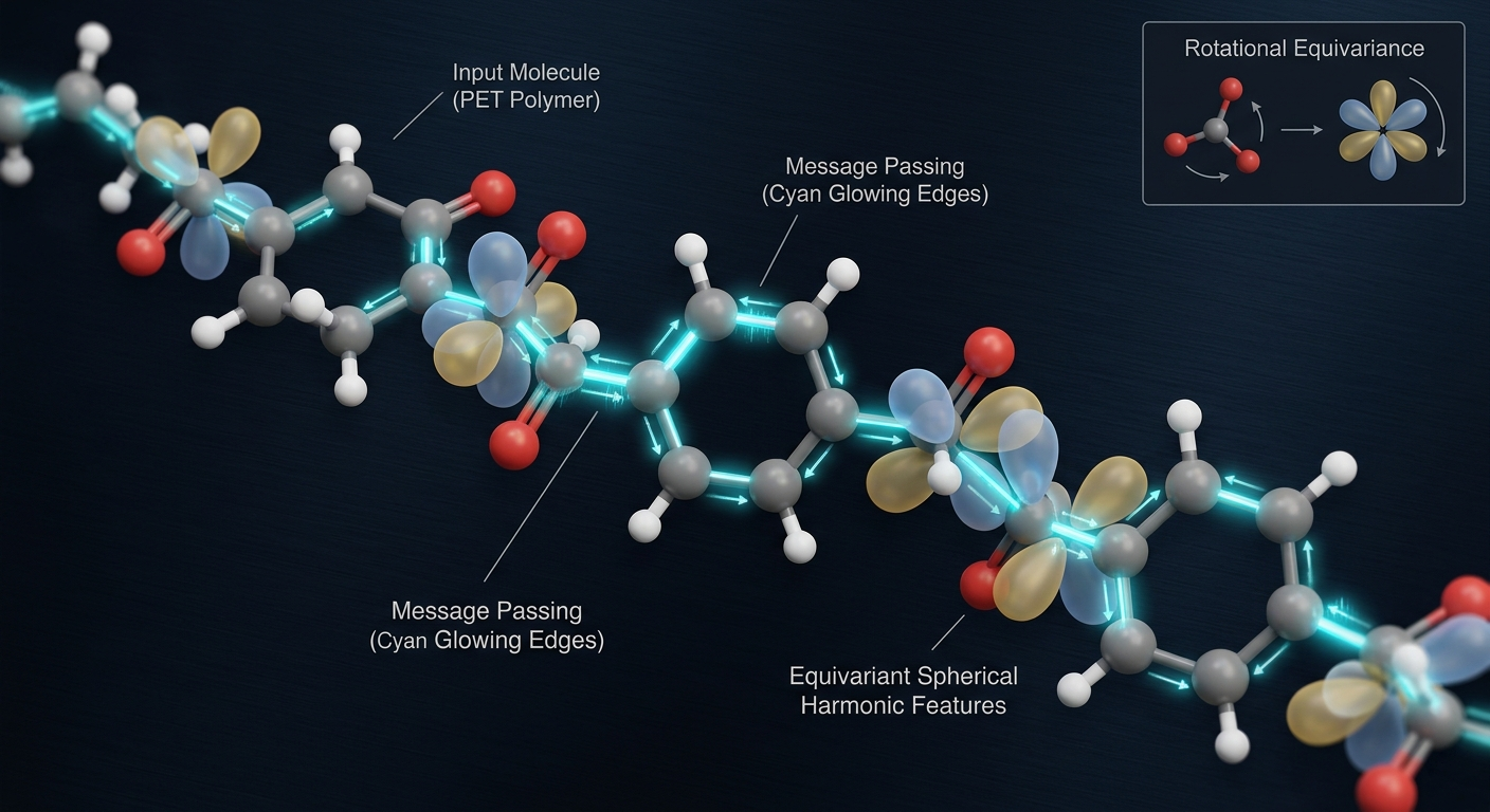
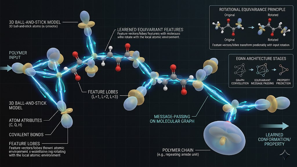
The first thing I had to figure out was the architecture. The wrong choice here is a standard feedforward network that takes Cartesian coordinates as input. Cartesian coordinates are not invariant to rotation and translation, which means a network trained that way would give different energy predictions for the same molecule in different orientations. That is physically wrong. The energy of a molecule does not depend on where it is sitting in space or which way it is pointing.

Equivariant networks solve this by building the rotational and translational symmetries into the architecture itself rather than hoping the training data covers all possible orientations. The way they do this is by representing each atom's environment as a set of features that transform predictably under rotation, using spherical harmonics as the basis. When you rotate the input, the internal representations rotate accordingly, and the output energy stays the same. I used a message-passing equivariant GNN where each atom is a node, edges connect atoms within a cutoff radius, and messages passed along edges encode the local chemical environment including bond distances and angles in an equivariant way.

Choosing the cutoff radius was less obvious than I expected. Too small and the network cannot see enough of the local environment to make accurate predictions, especially for a crosslinked polymer where stress distributes over relatively long length scales. Too large and the computational cost of the message-passing grows quickly. After testing a range from 4 to 8 angstroms, I settled on 6 angstroms as the right balance for epoxy-acid chemistry.

The training set construction was iterative. I started with the DFT data I already had from the Reformix pipeline, which covered equilibrium geometries and DFT-optimized structures at each polymerization stage. But a potential trained only on near-equilibrium configurations will fail when the MD simulation explores distorted geometries during bond formation, and it will fail badly, predicting nonsensical forces that send atoms flying apart or compressing unphysically.

The solution is active learning. You train a first-generation potential on the initial DFT data, then run MD using that potential and monitor the network's uncertainty on each configuration it encounters. When the uncertainty exceeds a threshold, that configuration is flagged, a single-point DFT calculation is run on it, and the result gets added to the training set. Then you retrain. Each cycle adds configurations from the parts of geometry space the simulation actually explores, and the potential gets progressively more reliable in exactly the regions that matter.

I ran four active learning cycles. The first generation potential was already good on equilibrium properties but fell apart above 400K, where the chains explore higher-energy configurations during annealing. By the third cycle it was stable across the full annealing temperature range. The fourth cycle added configurations from the biased MD runs specifically, so the potential could handle the stretched and compressed bond geometries that occur during the ring-opening reaction itself.

The validation benchmark I cared about was reproducing the Reformix results: density of 1.2975 g/cm³ at 300K, glass transition temperature of 76°C, Young's modulus of 4.36 GPa. These are the numbers that validated against experiment, so hitting them with the NNP instead of ReaxFF would confirm the potential is physically accurate and not just fitting to training data artifacts.

Density converged correctly by the second training cycle. Tg required the full four cycles, because getting the inflection point of the density-temperature curve right requires the potential to be accurate across the entire temperature range from 300K to 450K, not just at room temperature. The final modulus values were within the error bars of the ReaxFF results, which given the anisotropy of the finite simulation box is about as good as validation gets.

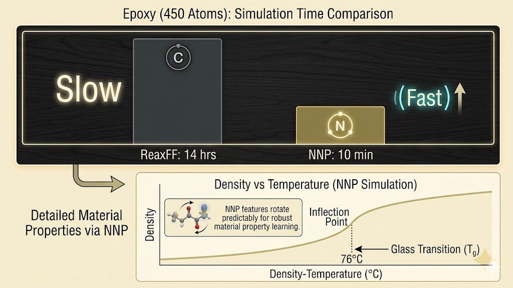
The speed difference on my hardware was around 80x for systems in the 400 to 500 atom range that Reformix uses. For larger systems, the gap grows wider. ReaxFF scales as roughly O(N²) because of the charge equilibration, and the NNP scales closer to O(N) once the neighbor list is built. Running a full Tg calculation that took 14 hours with ReaxFF now takes around 10 minutes.

That changes what is possible. At ReaxFF speed, screening 20 candidate formulations was a month of compute. At NNP speed, it is an afternoon. The screening engine becomes real.

The pipeline I built takes any set of DFT calculations on a molecular system, formats the data into the training schema, runs the active learning cycles automatically with configurable uncertainty thresholds, and outputs a trained potential ready to drop into a LAMMPS simulation. The only chemistry-specific input is the initial DFT dataset and the choice of cutoff radius. Everything else is automated.

The next step is extending the training set to cover a wider range of epoxy-acid chemistries beyond DGEBA-oxalic acid, so the potential generalizes across the formulation space Reformix is designed to screen rather than being specific to one validated system. That generalization is what turns this from a fast version of one simulation into a genuine screening engine.